From Riddles toRevelations- UnveilCaptivating TechStories and UnlockBusiness Growth!
Exposing all the expert insights to up-level your organization's brilliance.

Tech Talks & Insights
10 articles

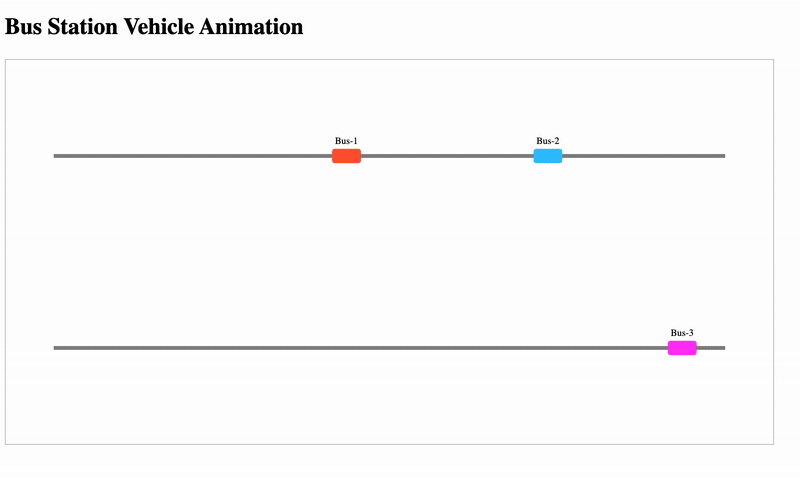
Animating Objects on a SVG Layout Using React and D3
Tracking and animating vehicles like buses, trains, or trams on a station map can be achieved using React + D3. In this tutorial, we demonstrate a generic approach using a bus example.We’ll create a hardcoded, self-contained project that shows buses moving along predefined tracks.Moving busesProject Structurebus-station-d3/├─ package.json├─ tsconfig.json├─ public/│ └─ index.html├─ src/│ ├─ App.tsx│ ├─ index.tsx│ ├─ hooks/│ │ └─ useBusMovement.ts│ └─ components/│ └─ BusStation.tsx├─ README.md2. Installationa. Create a React project:npx create-react-app bus-station-d3 --template typescriptcd bus-station-d3npm install d3 styled-componentsb. Copy the files into the src folder according to the structure above.3. Generic Vehicle Movement Hook (useBusMovement.ts)import { useEffect } from "react";import * as d3 from "d3";// Generic vehicles and station layoutconst VEHICLES = [ { id: 1, routeId: 1, position: 0 }, { id: 2, routeId: 1, position: 0.3 }, { id: 3, routeId: 2, position: 0.5 },];const STATION_LAYOUT = { width: 800, height: 400, tracks: [ { id: 1, start: { x: 50, y: 100 }, end: { x: 750, y: 100 } }, { id: 2, start: { x: 50, y: 300 }, end: { x: 750, y: 300 } }, ],};const COLORS = ["#FF5733", "#33C1FF", "#FF33F6"];export function useBusMovement({ containerRef }: { containerRef: any }) { useEffect(() => { if (!containerRef.current) return; const svg = d3 .select(containerRef.current) .append("svg") .attr("width", STATION_LAYOUT.width) .attr("height", STATION_LAYOUT.height); // Draw tracks STATION_LAYOUT.tracks.forEach((track) => { svg .append("line") .attr("x1", track.start.x) .attr("y1", track.start.y) .attr("x2", track.end.x) .attr("y2", track.end.y) .attr("stroke", "#888") .attr("stroke-width", 4); }); // Draw vehicles const vehicles = svg .selectAll(".vehicle") .data(VEHICLES) .enter() .append("g") .attr("class", (d) => `vehicle vehicle-${d.id}`); vehicles .append("rect") .attr("width", 30) .attr("height", 15) .attr("fill", (d, i) => COLORS[i % COLORS.length]) .attr("rx", 3) .attr("ry", 3); vehicles .append("text") .text((d) => `Bus-${d.id}`) .attr("x", 15) .attr("y", -5) .attr("text-anchor", "middle") .attr("font-size", 10) .attr("fill", "#000"); // Animate vehicles function animate() { VEHICLES.forEach((v) => { const track = STATION_LAYOUT.tracks.find((t) => t.id === v.routeId); if (!track) return; v.position += 0.002; if (v.position > 1) v.position = 0; const x = track.start.x + v.position * (track.end.x - track.start.x); const y = track.start.y + v.position * (track.end.y - track.start.y); svg.select(`.vehicle-${v.id}`).attr("transform", `translate(${x - 15},${y - 7.5})`); }); requestAnimationFrame(animate); } animate(); return () => svg.remove(); }, [containerRef]);}4. BusStation Component (BusStation.tsx)import { useRef } from "react";import { useBusMovement } from "../hooks/useBusMovement";import styled from "styled-components";const StationContainer = styled.div` width: 800px; height: 400px; border: 1px solid #ccc;`;export default function BusStation() { const containerRef = useRef<HTMLDivElement>(null); useBusMovement({ containerRef }); return <StationContainer ref={containerRef}></StationContainer>;}5. App Entry (App.tsx)import BusStation from "./components/BusStation";function App() { return ( <div className="App"> <h2>Bus Station Vehicle Animation</h2> <BusStation /> </div> );}export default App;6. Sample Images / DiagramTrack 1: ---------------------> (Bus 1 & 2)Track 2: ---------------------> (Bus 3)Rectangle = BusLine = TrackBuses move along the tracks in real-time.7. Run the Projectnpm installnpm start8. Key FeaturesGeneric VEHICLES object can represent buses, trams, or trains.All tracks and positions are hardcoded for simplicity.Animation runs with requestAnimationFrame for smooth movement.Easy to extend: Add stops, tooltips, or dynamic routes.Animating Objects on a SVG Layout Using React and D3 was originally published in IceApple Tech Talks on Medium, where people are continuing the conversation by highlighting and responding to this story.

How to start with terraform??
Prerequisite:Basic understanding of cloud concepts and hands on with any one of the cloud service like AWS, Azure, Google cloud.Visual studio codeWhat is Terraform?Terraform is an open-source tool created by HashiCorp. Terraform simplifies the cloud resource creation(Infrastructure as code) using the API’s given by the cloud provider. Terraform supports multiple cloud providers.Where to Start?Step 1: First install terraform tool from the hashicorp website (https://developer.hashicorp.com/terraform/install).Step 2: Create a directory and open it using Visual Studio Code.Step 3: Set up an AWS CLI profile that grants permission to provision resources. Initially, configure it with access keys and secrets for an administrator role.Steps 4: Create a basic and mandatory configuration file provider.tf to define which providers (like AWS, Azure, Google Cloud, etc.) your Terraform configuration will interact with. Basically all the terraform configuration files are created with .tf extension.provider sampleIn the provided configuration, the required_version property defines the minimum version of Terraform required, while required_providers specifies the specific cloud provider being utilized. Within the provider block, settings for the AWS CLI profile and region are specified, which dictate the configuration used for resource creation. Specify the profile name which we created in the previous step.Steps 5: Create a main.tf file and add a configuration to create an AWS S3 bucket. Terraform’s configuration language is declarative, we can refer the resource configuration syntax from Hashicorp documentation (https://registry.terraform.io/providers/hashicorp/aws/latest/docs ).Provided s3 resource configuration sample. resource blocks used to define the components.main.tfHow to run?The basic commands used to execute the terraform configurtions are terraform init, terraform validate, terraform fmt, terraform apply, terraform destroy.terraform init: When you create a new configuration or check out an existing configuration from version control you need to initialize the directory. Terraform downloads and installs the providers defined in the configuration in a subdirectory of your current working directory, named .terraform. In our case aws provider installed. Terraform also creates a lock file named .terraform.lock.hcl which specifies the exact provider versions used.terraform validate: It validates the configuration is syntactically valid and internally consistent.terraform fmt: Automatically format and update the configurations in the current directory for readability and consistency.terraform apply: Apply the configuration and creates the infrastructure. Before it applies any changes, Terraform prints out the execution plan which describes the actions Terraform will take in order to change your infrastructure to match the configuration. Execution plan can be printed using terraform plan command as well. Terraform wrote data into a file called terraform.tfstate. Terraform stores the IDs and properties of the resources it manages, so that it can update or destroy those resources going forward. State file is the only way Terraform can track which resources it manages, and often contains sensitive information, so you must store your state file securely.terraform destroy: This command terminates resources managed by your Terraform project. It terminates all the resources specified in your Terraform state. It does not destroy resources running elsewhere that are not managed by the current Terraform project.The commands described above can be executed sequentially to create an S3 bucket using the specified profile. Below are some example responses from these commands.Response sample for referenceIn the upcoming blog post, I’ll cover the configuration of modules, input and output variables, module organization, and the management of different environments etc.How to start with terraform?? was originally published in IceApple Tech Talks on Medium, where people are continuing the conversation by highlighting and responding to this story.

Tuning LLM: Exploring the Nuances of Prompt Tuning and Fine Tuning
Large Language Models (LLMs) have revolutionized the field of artificial intelligence, showing remarkable capabilities in understanding and generating human-like text. The ability of these models to perform a wide array of tasks, from casual conversations to complex problem-solving, is largely attributed to their sophisticated training methodologies. However, the performance of LLMs can often be enhanced through various tuning strategies.In the previous blog, we gained a basic understanding of prompt engineering and prompt tuning.What is Prompt? What is Prompt Engineering & Prompt Tuning?In this Blog, we delve into the nuances of prompting and fine-tuning, shedding light on how each method contributes to optimizing LLMs.Prompt Tuning: Influencing Outputs with InputsUnlike Prompt Engineering adding task-specific instructions along with the input, Here we introduce Soft Prompts, Soft prompts are task-specific instruction prompts, which are embedded in the input embedding layer of the model to guide towards desired behaviors and require minimal training at the input embedding layer by freezing the original weights of the model. Soft prompts are learned continuous embeddings, which are not necessarily interpretable as natural language but are used as input to the model. In simple, the soft prompts play a pivot role in how the input is presented to the model, This soft prompt embedding layer is learnable, In each iteration of training the soft prompt gets optimized over time.Strategies for Crafting Effective PromptsClarity and Conciseness: Clear and straightforward prompts are typically more effective than vague or overly complex ones. Aim for simplicity while keeping essential details.Contextual Framing: Providing context can improve the model’s ability to understand the desired output. Including examples or specific details can clarify the task.Iterative Refinement: Experiment with various prompts to determine which produces the best results. Tuning prompts involves iterative trial and error.Use of Instructional Language: Directly phrasing prompts as instructions, like “List the benefits of…”, can more effectively guide the model’s output.Benefits of Prompt TuningRapid Adaptation: Prompt tuning allows for quick adjustments to the model’s behavior without requiring extensive retraining, making it ideal for dynamic and real-time applications.Cost-Effective: Since it doesn’t involve large-scale data processing or lengthy training sessions, prompt tuning is a more cost-effective way to fine-tune models for specific tasks.Versatility: Prompt tuning can be applied across various domains and tasks, offering a flexible approach to customizing model outputs for different applications and contexts.Reduced Computational Resources: Compared to full model retraining, prompt tuning requires fewer computational resources, making it feasible for use on less powerful hardware.Let’s now dive into the coding, we can look into a sample Python code and see where this prompt tuning takes place for code generation tasks using soft prompts.import csvimport nltkimport randomfrom nltk.corpus import stopwordsfrom nltk.tokenize import word_tokenizeimport stringimport torchfrom tqdm import tqdmfrom torch.nn.utils.rnn import pad_sequenceimport torch.nn as nnfrom transformers import GPT2LMHeadModel, GPT2Tokenizer,GPT2Model, GPT2Config, AdamWfrom sklearn.model_selection import train_test_splitfirst, we import the required modulesdef preprocess_text(input_text): """ Processes the given text by converting it to lowercase, removing punctuation and digits, tokenizing the words, and filtering out stop words. Args: input_text (str): Text that needs to be processed. Returns: str: The processed text. """ # Convert text to lowercase input_text = input_text.lower() # Remove punctuation and digits input_text = input_text.translate(str.maketrans('', '', string.punctuation + string.digits)) # Tokenize the text into words words = word_tokenize(input_text) # Remove stop words filtered_words = [word for word in words if word not in stopwords.words('english')] # Join the words back into a single string processed_text = ' '.join(filtered_words) return processed_textwe gonna use a preprocessing function that would transform our text without stopping words and tokenizing.def tokenize_and_pad_sequences(data_pairs, max_len_article, max_len_highlights): """ Tokenizes the input text data and pads the sequences to the given maximum lengths. Args: data_pairs (list): A list of tuples with each tuple containing an article and its corresponding highlights. max_len_article (int): The maximum length for article sequences. max_len_highlights (int): The maximum length for highlight sequences. Returns: list: A list of tuples containing tokenized and padded sequences for articles and highlights. """ processed_data = [] for article, highlights in data_pairs: # Tokenize and convert text to indices article_indices = tokenizer.encode(article, add_special_tokens=True) highlights_indices = tokenizer.encode(highlights, add_special_tokens=True) # Padding the sequences to the specified maximum lengths padded_article = torch.tensor(article_indices + [tokenizer.pad_token_id] * (max_len_article - len(article_indices))) padded_highlights = torch.tensor(highlights_indices + [tokenizer.pad_token_id] * (max_len_highlights - len(highlights_indices))) # Ensure both tokenized sequences are not empty if len(article_indices) > 0 and len(highlights_indices) > 0: processed_data.append((padded_article, padded_highlights)) return processed_dataAfter preprocessing, now we tokenize the input data, convert the tokens to indices using the GPT-2 tokenizer, and pad sequences to specified lengths.def load_data_from_csv(file_path): """ Reads a CSV file and extracts columns for articles and highlights. Args: file_path (str): Path to the CSV file. Returns: list: A list of tuples containing articles and highlights. """ data = [] with open(file_path, 'r', encoding='utf-8') as f: reader = csv.DictReader(f) for row in reader: article = row.get('article', '') highlights = row.get('highlights', '') data.append((article, highlights)) return data# Load test datatest_file_path = 'test.csv'test_data = load_data_from_csv(test_file_path)# Load training datatrain_file_path = 'train.csv'train_data = load_data_from_csv(train_file_path)# Load validation datavalidation_file_path = 'validation.csv'validation_data = load_data_from_csv(validation_file_path)Here comes the dataset loading part, we try to read data from CSV files, extracting relevant columns (‘article’ and ‘highlights’) and storing them as tuples in separate lists for training, testing, and validation data.def sample_one_percent(data_list, seed): """ Randomly samples 1% of the data from the provided list for reproducibility. Args: data_list (list): The original data list. seed (int): Seed value for reproducibility. Returns: list: A list containing 1% of the sampled data. """ random.seed(seed) sample_size = int(0.01 * len(data_list)) return random.sample(data_list, sample_size)# Sample 1% of the test dataone_percent_test_data = sample_one_percent(test_data, seed=14)# Sample 1% of the training dataone_percent_train_data = sample_one_percent(train_data, seed=14)# Sample 1% of the validation dataone_percent_val_data = sample_one_percent(validation_data, seed=14)We randomly select 1% of the data from the training, testing, and validation datasets for effective processing during model building.# Apply preprocessing to the sampled dataprocessed_train_data = [(preprocess_text(article), preprocess_text(highlights)) for article, highlights in one_percent_train_data]processed_test_data = [(preprocess_text(article), preprocess_text(highlights)) for article, highlights in one_percent_test_data]processed_val_data = [(preprocess_text(article), preprocess_text(highlights)) for article, highlights in one_percent_val_data]This block processes the sampled data for the training, testing, and validation sets by applying text preprocessing (lowercasing, punctuation removal, tokenization, and stop word removal).# Initialize GPT-2 tokenizertokenizer = GPT2Tokenizer.from_pretrained("gpt2")# Set the padding token to the end-of-sequence token and add it to the tokenizerpad_token = tokenizer.eos_tokentokenizer.add_special_tokens({'pad_token': pad_token})# Define maximum lengths for articles and highlightsmax_article_len = 1021max_highlights_len = 1024# Apply tokenization and padding to the preprocessed datasetstokenized_train_data = tokenize_and_pad_sequences(processed_train_data, max_len_article=max_article_len, max_len_highlights=max_highlights_len)tokenized_test_data = tokenize_and_pad_sequences(processed_test_data, max_len_article=max_article_len, max_len_highlights=max_highlights_len)tokenized_val_data = tokenize_and_pad_sequences(processed_val_data, max_len_article=max_article_len, max_len_highlights=max_highlights_len)The GPT-2 tokenizer is loaded in this block, which also adds a unique token (“<pad>’’) to the tokenizer that will be used for padding sequences. Tokenized and padded datasets for training, testing, and validation are produced by this block by tokenizing and padding the preprocessed data to the designated maximum lengths for articles and highlights.# Initialize lists to store input and target IDs for training datainput_ids_train = []target_ids_train = []# Maximum lengths for articles and highlightsmax_article_len = 1021max_highlights_len = 1024# Iterate over the tokenized training datafor article_tokens, highlights_tokens in tokenized_train_data: # Truncate article tokens to the maximum article length truncated_article = article_tokens[:max_article_len] # Truncate highlights tokens to the maximum highlights length truncated_highlights = highlights_tokens[:max_highlights_len] # Add the truncated article tokens to the input list input_ids_train.append(truncated_article) # Add the truncated highlights tokens to the target list target_ids_train.append(truncated_highlights)# Convert training lists to PyTorch tensorsinput_ids_train = torch.stack(input_ids_train)target_ids_train = torch.stack(target_ids_train)This section trims the article and highlights tokens that are longer than the allowed limits before converting them into PyTorch tensors to prepare the training data.input_ids_val = []target_ids_val = []# Iterate over the tokenized validation datafor article_tokens, highlights_tokens in tokenized_val_data: # Truncate article tokens to the maximum article length truncated_article = article_tokens[:max_article_len] # Truncate highlights tokens to the maximum highlights length truncated_highlights = highlights_tokens[:max_highlights_len] # Add the truncated article tokens to the input list for validation input_ids_val.append(truncated_article) # Add the truncated highlights tokens to the target list for validation target_ids_val.append(truncated_highlights)# Convert validation lists to PyTorch tensorsinput_ids_val = torch.stack(input_ids_val)target_ids_val = torch.stack(target_ids_val)Similarly, we reduce the tokens for the validation set also and create PyTorch tensors# Load the GPT-2 model and tokenizermodel_name = "gpt2"tokenizer = GPT2Tokenizer.from_pretrained(model_name)gpt2_model = GPT2LMHeadModel.from_pretrained(model_name)# Define the number of prompt tokens and the embedding sizenum_prompt_tokens = 3 # For example, "summarize the following text"embedding_dim = gpt2_model.config.hidden_size# Specify the prompt sentenceprompt_sentence = "summarize"# Tokenize the prompt sentenceprompt_ids = tokenizer.encode(prompt_sentence, return_tensors='pt')# Obtain embeddings for the tokenized prompt sentence from the GPT-2 modelprompt_embeddings = gpt2_model.transformer.wte(prompt_ids)# Initialize an embedding layer for soft prompts with the prompt sentence embeddingssoft_prompt_layer = nn.Embedding(num_prompt_tokens, embedding_dim)soft_prompt_layer.weight.data.copy_(prompt_embeddings.squeeze(0))The GPT-2 model and tokenizer are loaded in this section. Tokenizing a particular sentence, retrieving embeddings from the GPT-2 model, initializing an embedding layer for soft prompts with the sentence embeddings, and defining the number of tokens in prompt and embedding size are all done inside this phase.class GPT2WithPromptTuning(nn.Module): def __init__(self, gpt2_model, soft_prompt_embeddings): super(GPT2WithPromptTuning, self).__init__() self.gpt2_model = gpt2_model self.soft_prompt_embeddings = soft_prompt_embeddings def forward(self, input_ids, soft_prompt_ids): # Obtain the embeddings for the input_ids from the GPT-2 model gpt2_embeddings = self.gpt2_model.transformer.wte(input_ids) # Obtain the embeddings for the soft prompts soft_prompt_embeds = self.soft_prompt_embeddings(soft_prompt_ids) # Concatenate the soft prompt embeddings with the input embeddings embeddings = torch.cat([soft_prompt_embeds, gpt2_embeddings], dim=1) # Pass the concatenated embeddings through the GPT-2 model outputs = self.gpt2_model(inputs_embeds=embeddings) return outputsThe one above concatenates soft prompt embeddings at the start of the input sequence, defining a unique GPT-2 model with prompt adjustments.# Initialize the modelmodel = GPT2WithPromptTuning(gpt2_model, soft_prompt_layer)# Freeze GPT-2 model weightsfor param in model.gpt2_model.parameters(): param.requires_grad = FalseHere we initiate the model with soft_promt_layer and also make the trainable parameters to freeze.# Define hyperparametersbatch_size = 8epochs = 2learning_rate = 2e-3gradient_clip_value = 1.0device = torch.device("cuda" if torch.cuda.is_available() else "cpu")# Move model to GPUmodel.to(device)# Define optimizer and criterionoptimizer = torch.optim.AdamW(model.soft_prompt_embeddings.parameters(), lr=learning_rate)criterion = nn.CrossEntropyLoss(ignore_index=-100)soft_prompt_ids = torch.tensor([0, 1, 2])This section initializes the AdamW optimizer and the cross-entropy loss function for training the model, as well as defines hyperparameters such as batch size, number of epochs, learning rate, and gradient clip value.# Training loopfor epoch in range(epochs): # Create a tqdm progress bar for the training data data_iterator = tqdm(zip(input_ids_train, target_ids_train), desc=f'Epoch {epoch + 1}', total=len(input_ids_train)) for input_ids, target_ids in data_iterator: optimizer.zero_grad() # Move input and target tensors to GPU input_ids, target_ids = input_ids.to(device), target_ids.to(device) outputs = model(input_ids, soft_prompt_ids.to(device)) logits = outputs.logits if hasattr(outputs, "logits") else outputs.last_hidden_state loss = criterion(logits, target_ids) loss.backward() # Gradient clipping to prevent exploding gradients torch.nn.utils.clip_grad_norm_(model.parameters(), gradient_clip_value) optimizer.step() # Update the progress bar description with the current loss data_iterator.set_postfix(loss=loss.item()) # Set the model back to training mode model.train()# Close the tqdm progress bardata_iterator.close()Here is an example of a sequence-to-sequence model’s training loop. Gradient descent is used in iterations over epochs to optimize the model’s parameters. To avoid gradient explosions, it computes the loss function, updates the model, and applies gradient clipping at each epoch.Fine-Tuning: The Model’s Weight Adjustment ApproachFine-tuning a Large Language Model (LLM) means adjusting or updating the pre-trained model parameters to improve performance over a specific task or domain. This process begins with a base model that was already trained on a huge dataset with a wide range of knowledge and linguistic patterns. During fine-tuning, the model is trained on the task-specific dataset, and its weights are adjusted using gradient descent to minimize the loss on this new dataset. This makes the model adapt its knowledge to effectively handle and understand the targeted task, such as summarization, question answering, code generation & debugging, or domain-specific text generation. By utilizing the vast knowledge gained from the pre-training phase, fine-tuning may significantly boost the model’s accuracy and relevance for particular tasks and create a balance between general understanding of language and specialized tasks.The Process of Fine-TuningDataset Preparation: A properly selected dataset that represents the target task is required for fine-tuning. For the model to effectively generalize, the chosen dataset should have a variety of contexts, styles, and approaches.Training Procedure: The model is trained on the new dataset, often for a reduced number of epochs. This training can be supervised (where correct outputs are provided) or unsupervised (learned from the data without explicit feedback).Evaluation and Adjustment: After fine-tuning, the model should be evaluated for performance on a validation set. Metrics such as accuracy, F1 score, or BLEU score can help gauge effectiveness. Based on these evaluations, further adjustments can be made.Benefits of Fine-TuningDomain Adaptation: Fine-tuning allows LLMs to specialize in niche domains, such as medical terminology or legal language, by adapting their understanding to specific jargon and context.Improved Performance: By training on relevant data, fine-tuned models often achieve better performance compared to their general-purpose counterparts.Flexibility: Fine-tuned models can efficiently handle a variety of tasks within their specialized domain, making them versatile for real-world applications.Let’s look at a sample Python code for Fine-Tuning GPT 2 LLM.import torchfrom torch.utils.data import DataLoaderfrom transformers import AutoTokenizer, AutoModelForCausalLM, Trainer, TrainingArgumentsfrom datasets import load_datasetdataset = load_dataset("wikitext", "wikitext-2-raw-v1")here we import the required libraries and load our wikitext-2 dataset, but you can use any dataset you prefer.model_name = "gpt2"tokenizer = AutoTokenizer.from_pretrained(model_name)def tokenize_function(examples): return tokenizer(examples["text"], padding="max_length", truncation=True)tokenized_datasets = dataset.map(tokenize_function, batched=True)Now we tokenized our dataset along with padding for fine-tuning.train_dataset = tokenized_datasets["train"]eval_dataset = tokenized_datasets["validation"]train_dataloader = DataLoader(train_dataset, shuffle=True, batch_size=8)eval_dataloader = DataLoader(eval_dataset, batch_size=8)Now we create DataLoaders for training and evaluation, DataLoaders ensure efficient and effective data handling during the training and evaluation of machine learning models. They help in batch processing, shuffling, parallel data loading, and better memory management, all of which contribute to more efficient training and evaluation processes.model = AutoModelForCausalLM.from_pretrained(model_name)training_args = TrainingArguments( output_dir="./results", evaluation_strategy="epoch", learning_rate=2e-5, per_device_train_batch_size=8, per_device_eval_batch_size=8, num_train_epochs=3, weight_decay=0.01,)The code snippet loads a pre-trained causal language model using the AutoModelForCausalLM class from the Hugging Face Transformers library. It then sets up training arguments with specific parameters such as output directory, evaluation strategy, learning rate, batch sizes, number of training epochs, and weight decay using the TrainingArguments class.trainer = Trainer( model=model, args=training_args, train_dataset=train_dataset, eval_dataset=eval_dataset,)trainer.train()model.save_pretrained("./fine-tuned-model")tokenizer.save_pretrained("./fine-tuned-model")The code initializes a Trainer to fine-tune the loaded model using the specified training arguments and datasets, then trains the model and saves the fine-tuned model and tokenizer to a specified directory.Navigating the Challenges of Prompt Tuning and Fine-TuningPrompt tuning faces several challenges. One significant issue is achieving the right balance between specificity and generality; overly specific prompts can limit the model’s versatility, while too general prompts may not yield precise results. Additionally, prompt tuning requires a deep understanding of the model’s behavior and the nuances of natural language, which can be complex and time-consuming. Ensuring consistency across different contexts and managing unexpected or biased outputs are also critical challenges that need to be addressed to harness the potential of prompt tuning effectively.Fine-tuning may result in major improvements in model performance and accuracy, but it also raises some challenges. Overfitting is an important problem wherein the model may perform poorly on unseen or new data due to its heavy tuning on the training set. Furthermore, obtaining the right datasets may require a significant time.Real-Time Applications of Prompt Tuning & Fine TuningPrompt tuning is useful when users require specific kinds of responses without the need for extensive model re-training (Fine Tuning) and have limited resources. For example, in customer service chatbots, well-engineered soft prompts can streamline interactions, and ensure that responses align with customer questions. In creative writing aids, prompts can inspire imaginative outputs while maintaining a corresponding narrative style.In fields where precise language and terminology are essential, such as healthcare, finance, and education, fine-tuning is frequently used. For instance, a medical record-tuned LLM can help healthcare workers with report writing, patient history analysis, and prescription recommendation generation.Here are some example scenarios for real-time applications to help choose between prompt tuning and fine-tuningConclusionLarge language model tuning is not a one-size-fits-all process; the decision between fine-tuning and prompt tuning is based on the unique requirements and limitations of the given task. Every tuning technique has advantages and disadvantages of its own, so a developer must know when and how to use each one.By carefully navigating such conditions and utilizing LLMs for their fundamental flexibility as well as their capacity to adapt and function well in a range of scenarios, we may be able to reduce the gap between human intentions and machine understanding.Tuning LLM: Exploring the Nuances of Prompt Tuning and Fine Tuning was originally published in IceApple Tech Talks on Medium, where people are continuing the conversation by highlighting and responding to this story.

Mastering React State Management: From Basics to Advanced Techniques
State management is a cornerstone of building robust applications in React. As your application grows, effectively managing state becomes increasingly crucial. In this blog post, we’ll explore state management in React, starting from the basics with useState and progressing to advanced techniques like the Context API, Redux, and Redux Toolkit. We'll also discuss common problems associated with each stage and how to address them.Basic State Management with useStateReact’s useState hook is the simplest way to manage state in a functional component. It allows you to add state variables to your components easily.Example:import React, { useState } from 'react';function Counter() { const [count, setCount] = useState(0); return ( <div> <p>Count: {count}</p> <button onClick={() => setCount(count + 1)}>Increment</button> </div> );}export default Counter;useState is perfect for managing simple, localized state. However, as your application grows, you might encounter the issue of prop drilling.Prop Drilling ProblemProp drilling occurs when you pass state and functions down through multiple layers of components. This can make your code harder to read and maintain.Example:function App() { const [user, setUser] = useState({ name: 'John', age: 30 }); return <Profile user={user} />;}function Profile({ user }) { return <ProfileDetails user={user} />;}function ProfileDetails({ user }) { return <p>{user.name}</p>;}As you can see, the user prop needs to be passed through each component even if it is not directly used by them. This is where the Context API comes in handy.Solving Prop Drilling with Context APIThe Context API provides a way to share values like state across the component tree without passing props down manually at every level.Example:import React, { createContext, useContext, useState } from 'react';const UserContext = createContext();function App() { const [user, setUser] = useState({ name: 'John', age: 30 }); return ( <UserContext.Provider value={user}> <Profile /> </UserContext.Provider> );}function Profile() { return <ProfileDetails />;}function ProfileDetails() { const user = useContext(UserContext); return <p>{user.name}</p>;}While the Context API is powerful for solving prop drilling, it can become cumbersome when dealing with complex state logic and updates. This is where Redux comes into play.Advanced State Management with ReduxRedux is a popular library for managing global state in a predictable way. It adheres to the principles of having a single source of truth, state being read-only, and changes being made with pure functions.Problems with Context API:Complexity in Updates: Managing complex state logic with the Context API can lead to deeply nested providers and consumers, making the code harder to follow.Performance Issues: Frequent state updates can lead to unnecessary re-renders of components consuming the context.Example:// actions.jsexport const increment = () => ({ type: 'INCREMENT' });// reducer.jsconst initialState = { count: 0 };function counterReducer(state = initialState, action) { switch (action.type) { case 'INCREMENT': return { ...state, count: state.count + 1 }; default: return state; }}// store.jsimport { createStore } from 'redux';import counterReducer from './reducer';const store = createStore(counterReducer);// App.jsimport React from 'react';import { Provider, useSelector, useDispatch } from 'react-redux';import store from './store';import { increment } from './actions';function Counter() { const count = useSelector((state) => state.count); const dispatch = useDispatch(); return ( <div> <p>Count: {count}</p> <button onClick={() => dispatch(increment())}>Increment</button> </div> );}function App() { return ( <Provider store={store}> <Counter /> </Provider> );}export default App;Simplifying Redux with Redux ToolkitRedux Toolkit is the official, opinionated, and batteries-included toolset for efficient Redux development. It simplifies the configuration and reduces boilerplate code.Example:// store.jsimport { configureStore, createSlice } from '@reduxjs/toolkit';const counterSlice = createSlice({ name: 'counter', initialState: { count: 0 }, reducers: { increment: (state) => { state.count += 1; }, },});const store = configureStore({ reducer: counterSlice.reducer,});export const { increment } = counterSlice.actions;export default store;// App.jsimport React from 'react';import { Provider, useSelector, useDispatch } from 'react-redux';import store, { increment } from './store';function Counter() { const count = useSelector((state) => state.count); const dispatch = useDispatch(); return ( <div> <p>Count: {count}</p> <button onClick={() => dispatch(increment())}>Increment</button> </div> );}function App() { return ( <Provider store={store}> <Counter /> </Provider> );}export default App;Additional Topics in Redux ToolkitRedux Toolkit provides several advanced features that make state management even more powerful and efficient.Async ThunkRedux Toolkit includes createAsyncThunk, which simplifies handling asynchronous actions like fetching data from an API. It helps manage the lifecycle of an async request by generating action types for pending, fulfilled, and rejected states. This reduces the boilerplate code and makes it easier to handle loading states and errors within your application.Example:// store.jsimport { configureStore, createSlice, createAsyncThunk } from '@reduxjs/toolkit';import axios from 'axios';export const fetchUser = createAsyncThunk('user/fetchUser', async (userId) => { const response = await axios.get(`/api/user/${userId}`); return response.data;});const userSlice = createSlice({ name: 'user', initialState: { user: null, status: 'idle' }, reducers: {}, extraReducers: (builder) => { builder .addCase(fetchUser.pending, (state) => { state.status = 'loading'; }) .addCase(fetchUser.fulfilled, (state, action) => { state.status = 'succeeded'; state.user = action.payload; }) .addCase(fetchUser.rejected, (state) => { state.status = 'failed'; }); },});const store = configureStore({ reducer: userSlice.reducer,});export default store;Mutating StateOne of the notable features of Redux Toolkit is that it uses Immer under the hood. This allows you to write “mutating” logic in reducers, which actually produces immutable updates. Immer provides a draft state that can be mutated directly without affecting the original state. When the mutations are complete, Immer produces a new immutable state based on the changes made to the draft state.Example:const counterSlice = createSlice({ name: 'counter', initialState: { count: 0 }, reducers: { increment: (state) => { state.count += 1; }, },});ConclusionEffective state management is key to building scalable React applications. Starting with useState for simple cases, you can address prop drilling with the Context API. For more complex state logic and global state management, Redux and Redux Toolkit provide powerful solutions. With features like async thunks, middleware, and the ability to write mutating logic safely, Redux Toolkit makes managing state in your React applications more efficient and maintainable.Learn more about Redux Toolkit here.Thanks for reading : ) Happy coding!Mastering React State Management: From Basics to Advanced Techniques was originally published in IceApple Tech Talks on Medium, where people are continuing the conversation by highlighting and responding to this story.
Understanding CSS Units: px, em, rem, %, vw, and vh
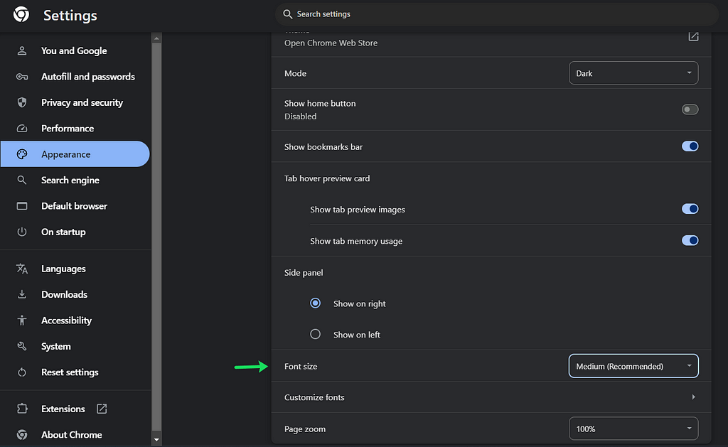
CSS units are the building blocks of web design, determining the sizing and spacing of elements. These units can be broadly categorized into two types: Absolute Units and Relative Units.Absolute UnitsAbsolute units have fixed values and are not affected by other elements. They include:Pixels (px): The most commonly used absolute unit, representing one dot on the screen.Inches (in), Centimeters (cm), Millimeters (mm): Physical units rarely used in web design.Points (pt) and Picas (pc): Units used primarily in print.Relative UnitsRelative units are flexible and scale according to other factors such as the font size of a parent element or the size of the viewport. They include:Ems (em) and Rems (rem): Relative to the font size of the parent and root elements, respectively.Percentages (%): Relative to the size of the parent element.Viewport Units (vw and vh): Relative to the size of the viewport.Now, let’s dive deeper into the most commonly used CSS units: pixels (px), ems (em), rems (rem), percentages (%), and viewport units (vw and vh).Pixels (px)Pixels are the most straightforward unit. One pixel (px) represents one dot on the screen. It’s an absolute unit, meaning it doesn’t change in size based on any other settings. For example:.element { font-size: 16px; margin: 20px;}Using pixels ensures that elements remain the same size regardless of the user’s settings. However, this lack of flexibility can be a drawback.Ems (em)Ems are relative units that scale based on the font size of their parent element. One em is equal to the current font size. If the parent element has a font size of 16px, 1em equals 16px. For example:.parent { font-size: 16px;}.child { font-size: 2em; /* 32px */ margin: 1em; /* 16px */}Using ems allows for scalable and adaptive designs, making it easier to maintain consistent proportions.Rems (rem)Rems (root ems) are similar to ems but are always relative to the root (html) element’s font size. This makes rems more predictable and easier to use for maintaining consistent spacing and sizing across your website. For example:html { font-size: 16px;}.element { font-size: 1.5rem; /* 24px */ padding: 1rem; /* 16px */}Using rems ensures that all sizes scale consistently based on the root font size, regardless of their nesting in the DOM.Percentages (%)Percentages are relative to the size of the parent element. They are often used for setting widths and heights:.container { width: 50%; /* 50% of the parent element's width */}.image { height: 80%; /* 80% of the parent element's height */}Percentages are useful for creating responsive designs that adapt to various screen sizes.Viewport Units (vw and vh)Viewport units are relative to the size of the browser’s viewport. 1vw is 1% of the viewport’s width, and 1vh is 1% of the viewport’s height. For example:.hero { width: 100vw; /* 100% of the viewport width */ height: 50vh; /* 50% of the viewport height */}Viewport units are particularly useful for full-screen elements and responsive designs that need to adapt to the user’s device.Why Use rem and em Instead of px?Using rem and em units over pixels has significant advantages, especially regarding accessibility and responsiveness:Scalability: Rem and em units scale based on the user’s settings. If a user increases the default font size in their browser for better readability, elements using rem and em units will scale accordingly, ensuring a consistent and accessible experience.Maintainability: Using relative units like rems and ems makes it easier to maintain and adjust your design. You can change the base font size, and all related sizes will adjust automatically.Example of Adjusting Font Size in ChromeIn Chrome, users can adjust the default font size in settings. If a website uses rem or em units, increasing the default font size will scale up the entire website, making it more accessible for users with visual impairments. Websites using pixels, however, will remain the same size, potentially causing readability issues.Above is an example of how changing the font size in browser settings impacts websites using rem and em units versus pixels. Notice how the site with rem/em units adapts to the larger font size, while the one using pixels does not.ConclusionUnderstanding and effectively using CSS units is crucial for creating responsive and accessible web designs. While pixels offer precision, rems, and ems provide flexibility and scalability, ensuring your website adapts to various user settings and devices. By using relative units, you create a more user-friendly and maintainable design, enhancing the overall user experience.Thanks for reading : ) Happy coding!Understanding CSS Units: px, em, rem, %, vw, and vh was originally published in IceApple Tech Talks on Medium, where people are continuing the conversation by highlighting and responding to this story.
Showing 6 of 10 articles

Let's Build Together
Feeling Inspired?
Share your vision and our experts will get back to you within 24 hours.
- Expert team with 10+ years of experience
- Custom solutions tailored to your business
- End-to-end support from concept to delivery
- Trusted by 100+ global clients